Mapping Tools
geopandas provides a high-level interface to the matplotlib library for making maps. Mapping shapes is as easy as using the plot() method on a GeoSeries or GeoDataFrame.
Loading some example data:
In [1]: world = gpd.read_file(gpd.datasets.get_path('naturalearth_lowres'))

In [2]: cities = gpd.read_file(gpd.datasets.get_path('naturalearth_cities'))
We can now plot those GeoDataFrames:
# Examine country GeoDataFrame
In [3]: world.head()
Out[3]:
       continent  gdp_md_est  \
0           Asia     22270.0
1         Africa    110300.0
2         Europe     21810.0
3           Asia    184300.0
4  South America    573900.0

                                            geometry iso_a3  \
0  POLYGON ((61.21081709172574 35.65007233330923,...    AFG
1  (POLYGON ((16.32652835456705 -5.87747039146621...    AGO
2  POLYGON ((20.59024743010491 41.85540416113361,...    ALB
3  POLYGON ((51.57951867046327 24.24549713795111,...    ARE
4  (POLYGON ((-65.50000000000003 -55.199999999999...    ARG

                   name     pop_est
0           Afghanistan  28400000.0
1                Angola  12799293.0
2               Albania   3639453.0
3  United Arab Emirates   4798491.0
4             Argentina  40913584.0

# Basic plot, random colors
In [4]: world.plot();
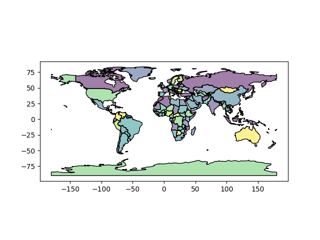
Note that in general, any options one can pass to pyplot in matplotlib (or style options that work for lines) can be passed to the plot() method.
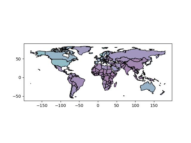
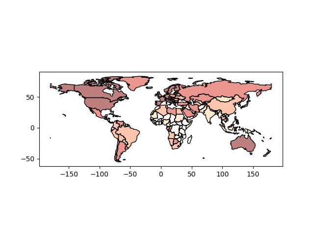
Chloropleth Maps
geopandas makes it easy to create Chloropleth maps (maps where the color of each shape is based on the value of an associated variable). Simply use the plot command with the column argument set to the column whose values you want used to assign colors.
# Plot by GDP per capta
In [5]: world = world[(world.pop_est>0) & (world.name!="Antarctica")]

In [6]: world['gdp_per_cap'] = world.gdp_md_est / world.pop_est

In [7]: world.plot(column='gdp_per_cap');
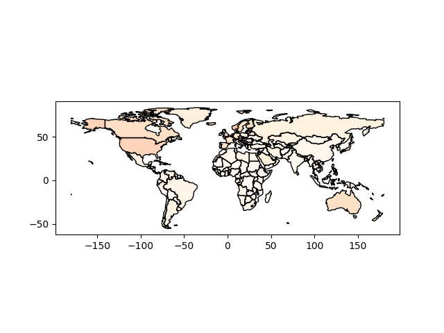
Choosing colors
One can also modify the colors used by plot with the cmap option (for a full list of colormaps, see the matplotlib website):
In [8]: world.plot(column='gdp_per_cap', cmap='OrRd');
The way color maps are scaled can also be manipulated with the scheme option (if you have pysal installed, which can be accomplished via conda install pysal). By default, scheme is set to ‘equal_intervals’, but it can also be adjusted to any other pysal option, like ‘quantiles’, ‘percentiles’, etc.
In [9]: world.plot(column='gdp_per_cap', cmap='OrRd', scheme='quantiles');
Maps with Layers
There are two strategies for making a map with multiple layers – one more succinct, and one that is a littel more flexible.
Before combining maps, however, remember to always ensure they share a common CRS (so they will align).
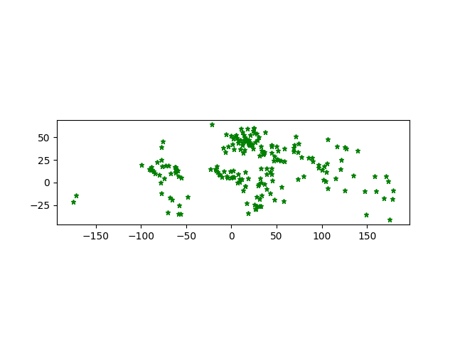
# Look at capitals
# Note use of standard `pyplot` line style options
In [10]: cities.plot(marker='*', color='green', markersize=5);
# Check crs
In [11]: cities = cities.to_crs(world.crs)
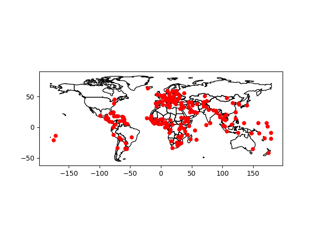
# Now we can overlay over country outlines
# And yes, there are lots of island capitals
# apparently in the middle of the ocean!
Method 1
In [12]: base = world.plot(color='white')

In [13]: cities.plot(ax=base, marker='o', color='red', markersize=5);

Method 2: Using matplotlib objects
In [14]: import matplotlib.pyplot as plt
In [15]: fig, ax = plt.subplots()
# set aspect to equal. This is done automatically
# when using *geopandas* plot on it's own, but not when
# working with pyplot directly.
In [16]: ax.set_aspect('equal')
In [17]: world.plot(ax=ax, color='white')
Out[17]: <matplotlib.axes._subplots.AxesSubplot at 0x7f27c95008d0>
In [18]: cities.plot(ax=ax, marker='o', color='red', markersize=5)
�������������������������������������������������������������������Out[18]: <matplotlib.axes._subplots.AxesSubplot at 0x7f27c95008d0>
In [19]: plt.show();