Set operations with overlay#
When working with multiple spatial datasets – especially multiple polygon or
line datasets – users often wish to create new shapes based on places where
those datasets overlap (or don’t overlap). These manipulations are often
referred using the language of sets – intersections, unions, and differences.
These types of operations are made available in the GeoPandas library through
the overlay() method.
The basic idea is demonstrated by the graphic below but keep in mind that
overlays operate at the DataFrame level, not on individual geometries, and the
properties from both are retained. In effect, for every shape in the left
GeoDataFrame, this operation is executed against every other shape in the right
GeoDataFrame:
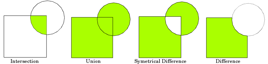
Source: QGIS documentation
Note
Note to users familiar with the shapely library: overlay() can be thought
of as offering versions of the standard shapely set operations that deal with
the complexities of applying set operations to two GeoSeries. The standard
shapely set operations are also available as GeoSeries methods.
The different overlay operations#
First, create some example data:
In [1]: from shapely.geometry import Polygon

In [2]: polys1 = geopandas.GeoSeries([Polygon([(0,0), (2,0), (2,2), (0,2)]),
   ...:                               Polygon([(2,2), (4,2), (4,4), (2,4)])])
   ...:

In [3]: polys2 = geopandas.GeoSeries([Polygon([(1,1), (3,1), (3,3), (1,3)]),
   ...:                               Polygon([(3,3), (5,3), (5,5), (3,5)])])
   ...:

In [4]: df1 = geopandas.GeoDataFrame({'geometry': polys1, 'df1':[1,2]})

In [5]: df2 = geopandas.GeoDataFrame({'geometry': polys2, 'df2':[1,2]})
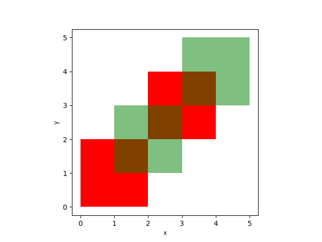
These two GeoDataFrames have some overlapping areas:
In [6]: ax = df1.plot(color='red');

In [7]: df2.plot(ax=ax, color='green', alpha=0.5);
The above example illustrates the different overlay modes.
The overlay() method will determine the set of all individual geometries
from overlaying the two input GeoDataFrames. This result covers the area covered
by the two input GeoDataFrames, and also preserves all unique regions defined by
the combined boundaries of the two GeoDataFrames.
Note
For historical reasons, the overlay method is also available as a top-level function overlay().
It is recommended to use the method as the function may be deprecated in the future.
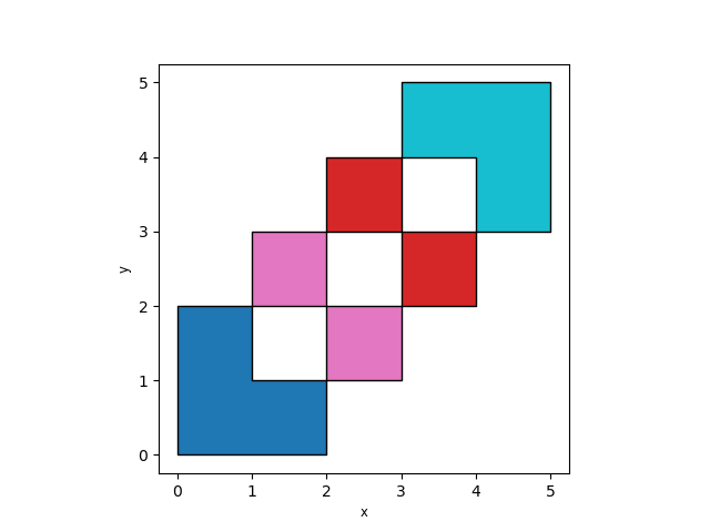
When using how='union', all those possible geometries are returned:
In [8]: res_union = df1.overlay(df2, how='union')

In [9]: res_union
Out[9]:
   df1  df2                                           geometry
0  1.0  1.0                POLYGON ((2 2, 2 1, 1 1, 1 2, 2 2))
1  2.0  1.0                POLYGON ((2 2, 2 3, 3 3, 3 2, 2 2))
2  2.0  2.0                POLYGON ((4 4, 4 3, 3 3, 3 4, 4 4))
3  1.0  NaN      POLYGON ((2 0, 0 0, 0 2, 1 2, 1 1, 2 1, 2 0))
4  2.0  NaN  MULTIPOLYGON (((3 4, 3 3, 2 3, 2 4, 3 4)), ((4...
5  NaN  1.0  MULTIPOLYGON (((2 3, 2 2, 1 2, 1 3, 2 3)), ((3...
6  NaN  2.0      POLYGON ((3 5, 5 5, 5 3, 4 3, 4 4, 3 4, 3 5))

In [10]: ax = res_union.plot(alpha=0.5, cmap='tab10')

In [11]: df1.plot(ax=ax, facecolor='none', edgecolor='k');

In [12]: df2.plot(ax=ax, facecolor='none', edgecolor='k');
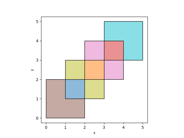
The other how operations will return different subsets of those geometries.
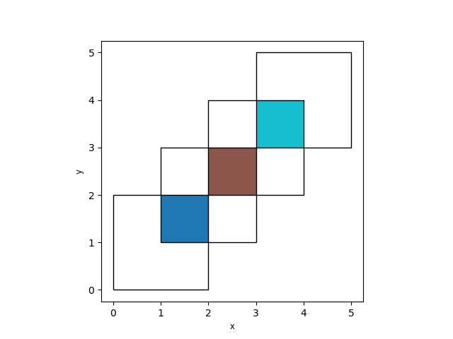
With how='intersection', it returns only those geometries that are contained
by both GeoDataFrames:
In [13]: res_intersection = df1.overlay(df2, how='intersection')

In [14]: res_intersection
Out[14]:
   df1  df2                             geometry
0    1    1  POLYGON ((2 2, 2 1, 1 1, 1 2, 2 2))
1    2    1  POLYGON ((2 2, 2 3, 3 3, 3 2, 2 2))
2    2    2  POLYGON ((4 4, 4 3, 3 3, 3 4, 4 4))

In [15]: ax = res_intersection.plot(cmap='tab10')

In [16]: df1.plot(ax=ax, facecolor='none', edgecolor='k');

In [17]: df2.plot(ax=ax, facecolor='none', edgecolor='k');
how='symmetric_difference' is the opposite of 'intersection' and returns
the geometries that are only part of one of the GeoDataFrames but not of both:
In [18]: res_symdiff = df1.overlay(df2, how='symmetric_difference')

In [19]: res_symdiff
Out[19]:
   df1  df2                                           geometry
0  1.0  NaN      POLYGON ((2 0, 0 0, 0 2, 1 2, 1 1, 2 1, 2 0))
1  2.0  NaN  MULTIPOLYGON (((3 4, 3 3, 2 3, 2 4, 3 4)), ((4...
2  NaN  1.0  MULTIPOLYGON (((2 3, 2 2, 1 2, 1 3, 2 3)), ((3...
3  NaN  2.0      POLYGON ((3 5, 5 5, 5 3, 4 3, 4 4, 3 4, 3 5))

In [20]: ax = res_symdiff.plot(cmap='tab10')

In [21]: df1.plot(ax=ax, facecolor='none', edgecolor='k');

In [22]: df2.plot(ax=ax, facecolor='none', edgecolor='k');
To obtain the geometries that are part of df1 but are not contained in
df2, you can use how='difference':
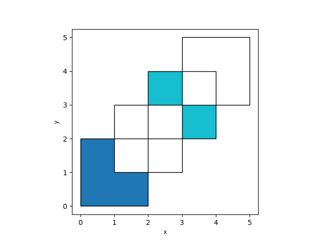
In [23]: res_difference = df1.overlay(df2, how='difference')

In [24]: res_difference
Out[24]:
                                            geometry  df1
0      POLYGON ((2 0, 0 0, 0 2, 1 2, 1 1, 2 1, 2 0))    1
1  MULTIPOLYGON (((3 4, 3 3, 2 3, 2 4, 3 4)), ((4...    2

In [25]: ax = res_difference.plot(cmap='tab10')

In [26]: df1.plot(ax=ax, facecolor='none', edgecolor='k');

In [27]: df2.plot(ax=ax, facecolor='none', edgecolor='k');
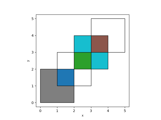
Finally, with how='identity', the result consists of the surface of df1,
but with the geometries obtained from overlaying df1 with df2:
In [28]: res_identity = df1.overlay(df2, how='identity')

In [29]: res_identity
Out[29]:
   df1  df2                                           geometry
0    1  1.0                POLYGON ((2 2, 2 1, 1 1, 1 2, 2 2))
1    2  1.0                POLYGON ((2 2, 2 3, 3 3, 3 2, 2 2))
2    2  2.0                POLYGON ((4 4, 4 3, 3 3, 3 4, 4 4))
3    1  NaN      POLYGON ((2 0, 0 0, 0 2, 1 2, 1 1, 2 1, 2 0))
4    2  NaN  MULTIPOLYGON (((3 4, 3 3, 2 3, 2 4, 3 4)), ((4...

In [30]: ax = res_identity.plot(cmap='tab10')

In [31]: df1.plot(ax=ax, facecolor='none', edgecolor='k');

In [32]: df2.plot(ax=ax, facecolor='none', edgecolor='k');
Overlay groceries example#
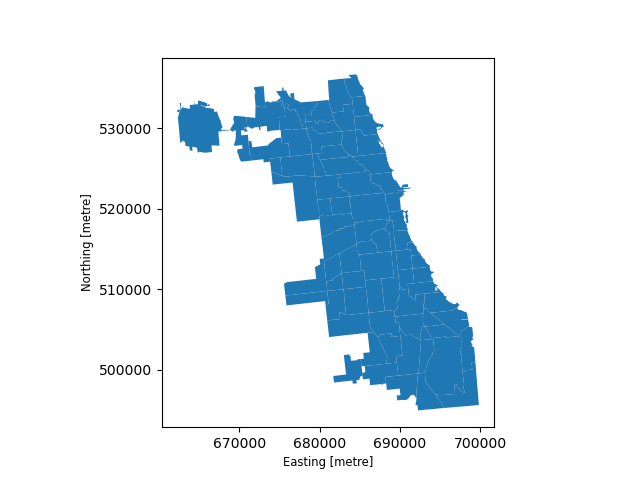
First, load the Chicago community areas and groceries example datasets and select :
In [33]: import geodatasets

In [34]: chicago = geopandas.read_file(geodatasets.get_path("geoda.chicago_commpop"))

In [35]: groceries = geopandas.read_file(geodatasets.get_path("geoda.groceries"))

# Project to crs that uses meters as distance measure
In [36]: chicago = chicago.to_crs("ESRI:102003")

In [37]: groceries = groceries.to_crs("ESRI:102003")
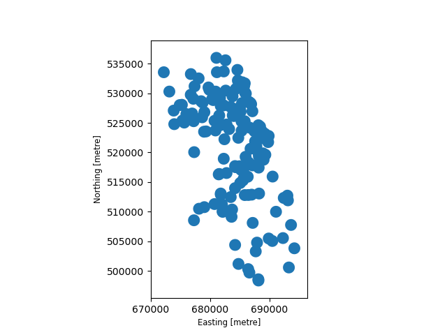
To illustrate the overlay() method, consider the following case in which one
wishes to identify the “served” portion of each area – defined as areas within
1km of a grocery store – using a GeoDataFrame of community areas and a
GeoDataFrame of groceries.
# Look at Chicago:
In [38]: chicago.plot();
# Now buffer groceries to find area within 1km.
# Check CRS -- USA Contiguous Albers Equal Area, units of meters.
In [39]: groceries.crs
Out[39]:
<Projected CRS: ESRI:102003>
Name: USA_Contiguous_Albers_Equal_Area_Conic
Axis Info [cartesian]:
- E[east]: Easting (metre)
- N[north]: Northing (metre)
Area of Use:
- name: United States (USA) - CONUS onshore - Alabama; Arizona; Arkansas; California; Colorado; Connecticut; Delaware; Florida; Georgia; Idaho; Illinois; Indiana; Iowa; Kansas; Kentucky; Louisiana; Maine; Maryland; Massachusetts; Michigan; Minnesota; Mississippi; Missouri; Montana; Nebraska; Nevada; New Hampshire; New Jersey; New Mexico; New York; North Carolina; North Dakota; Ohio; Oklahoma; Oregon; Pennsylvania; Rhode Island; South Carolina; South Dakota; Tennessee; Texas; Utah; Vermont; Virginia; Washington; West Virginia; Wisconsin; Wyoming.
- bounds: (-124.79, 24.41, -66.91, 49.38)
Coordinate Operation:
- name: USA_Contiguous_Albers_Equal_Area_Conic
- method: Albers Equal Area
Datum: North American Datum 1983
- Ellipsoid: GRS 1980
- Prime Meridian: Greenwich
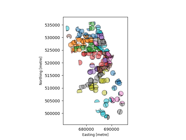
# make 1km buffer
In [40]: groceries['geometry']= groceries.buffer(1000)
In [41]: groceries.plot();
To select only the portion of community areas within 1km of a grocery, specify the how option to be “intersect”, which creates a new set of polygons where these two layers overlap:
In [42]: chicago_cores = chicago.overlay(groceries, how='intersection')

In [43]: chicago_cores.plot(alpha=0.5, edgecolor='k', cmap='tab10');
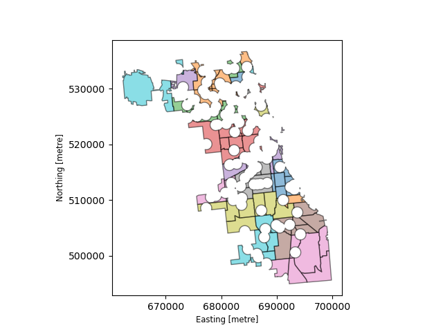
Changing the how option allows for different types of overlay operations. For example, if you were interested in the portions of Chicago far from groceries (the peripheries), you would compute the difference of the two.
In [44]: chicago_peripheries = chicago.overlay(groceries, how='difference')

In [45]: chicago_peripheries.plot(alpha=0.5, edgecolor='k', cmap='tab10');
keep_geom_type keyword#
In default settings, overlay() returns only geometries of the same geometry type as GeoDataFrame
(left one) has, where Polygon and MultiPolygon is considered as a same type (other types likewise).
You can control this behavior using keep_geom_type option, which is set to
True by default. Once set to False, overlay will return all geometry types resulting from
selected set-operation. Different types can result for example from intersection of touching geometries,
where two polygons intersects in a line or a point.
More examples#
A larger set of examples of the use of overlay() can be found here